Probability,

Factorial numbers (written as n!)) are primarily used to count the total number of ways to arrange a specific group of items. They are used in mathematics, computer science, and statistics for calculating possibilities, probabilities, and system efficiencies.
By convention ! =1
1! = 1    2! = 2x1 =2         3! = 3x2x1 = 6     4! = 4x3x2x1 = 24     5! =5x4x3x2x1 =120     6! = 6x5x4x3x2x1=720
The most direct use of a factorial is finding how many unique orders or sequences can be made from a set. 
Lineups: Arranging 4 people in a single file line: 4! ways (24)  
Scheduling: Ordering 5 tasks on a daily to-do list: 5! ways (120)
Travel: Finding the total possible routes to visit 8 distinct cities: 8! routes 
Card Games: Shuffling a standard 52-card deck yields 52!

To convert a number from the factorial number to an ordinary number , you must multiply each digit by its corresponding positional factorial value and then add the results together.

Fibonacci sequences and The Golden Ratio.

The Fibonacci sequence is a sequence in which each element is the sum of the two elements that precede it. Numbers that are part of the Fibonacci sequence are known as Fibonacci numbers, commonly denoted Fn .
Starting from 0 and 1, the sequence begins:  0, 1, 1, 2, 3, 5, 8, 13, 21, 34, 55, 89, 144, ...
The ratio of one Fn divided by the preceding Fn  tend to  be 1.618, the golden ratio.

The Fibonacci numbers were first described in Indian mathematics as early as 200 BC in work by Pingala on enumerating possible patterns of Sanskrit poetry formed from syllables of two lengths. They are named after the Italian mathematician Leonardo of Pisa, also known as Fibonacci, who introduced the sequence to Western European mathematics in his 1202 book Liber Abaci.

The ratio of one number divided by the preceding one tends to the golden ratio of 1.618.
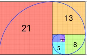
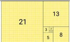
A golden rectangle has its sides in the golden ratio. If a rectangle is a golden rectangle, any new rectangle created by adding or removing a square from the golden rectangle, will also be a golden rectangle:

Fibonacci tiling with squares whose side lengths are successive Fibonacci numbers: 1, 1, 2, 3, 5, 8, 13 and 21

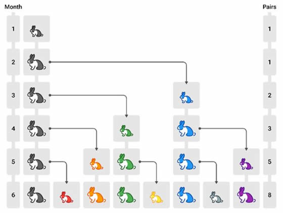
Solution to the  Fibonacci rabbit problem: The Fibonacci rabbit problem is a famous mathematical thought experiment introduced by Italian mathematician Leonardo of Pisa (Fibonacci) in his 1202 book, Liber Abaci . It is the historical origin of the Fibonacci sequence in Western mathematics. In a growing idealized population, the number of rabbit pairs form the Fibonacci sequence. At the end of the nth month, the number of pairs is equal to Fn.
Fibonacci posed the rabbit math problem: how many pairs will there be in one year?

At the end of the first month, they mate, but there is still only 1 pair.
At the end of the second month they produce a new pair, so there are 2 pairs in the field.
At the end of the third month, the original pair produce a second pair, but the second pair only mate to gestate for a month, so there are 3 pairs in all.
At the end of the fourth month, the original pair has produced yet another new pair, and the pair born two months ago also produces their first pair, making 5 pairs.
At the end of the n-th month, the number of pairs of rabbits is equal to the number of mature pairs (that is, the number of pairs in month n – 2) plus the number of pairs alive last month (month n – 1). The number in the n-th month is the n-th Fibonacci number.

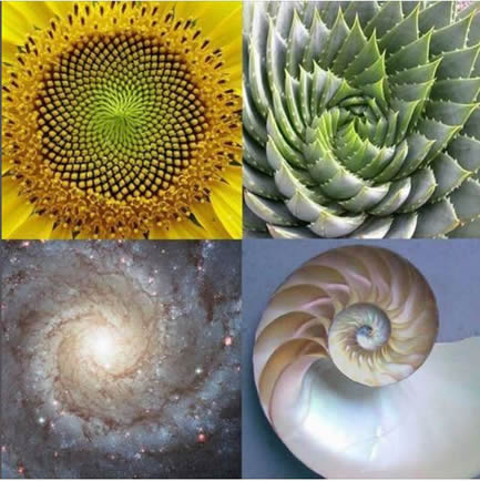
• Sunflowers and Daisies: The seeds in a sunflower head are packed in two sets of interlocking spirals—one clockwise and one counterclockwise. If you count the spirals, the totals are almost always consecutive Fibonacci numbers, typically 21 and 34, 34 and 55, or 55 and 89.

• Pinecones and Pineapples: The scales of a pinecone or the sections of a pineapple form steep spirals. Counting these parallel rows typically yields Fibonacci numbers like 8 and 13.

• Phyllotaxis (Leaf Arrangement): As stems grow, leaves sprout at a fraction of a turn relative to the previous leaf. This angle (the Golden Angle, roughly 137.5 degrees) ensures that newer leaves never perfectly block older ones from receiving sunlight.

• Romanesco Broccoli: This vegetable is a striking visual example of a natural fractal. Each bud is arranged in a Fibonacci spiral, and every individual bud is itself a miniature version of the larger spiral.

The Growth Spiral
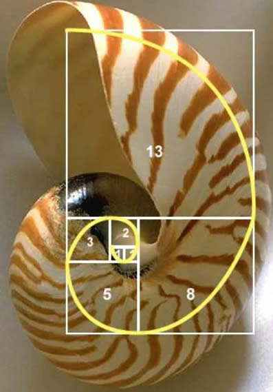
This shape allows an organism to grow larger without changing its proportions, as seen in the chambers of a Nautilus shell, the unfurling of a fern fiddlehead, or the swirling arms of a hurricane.

Probability

When looking at multiple events, the rules depend entirely on whether the
events affect each other.

To find a missing probability from a probability distribution table.

Let's take a look at the following example:Another handy time to use this rule is to find a missing

In this table, the "X" column denotes the possible outcomes. The "Probability" column denotes the probability of achieving each outcome.

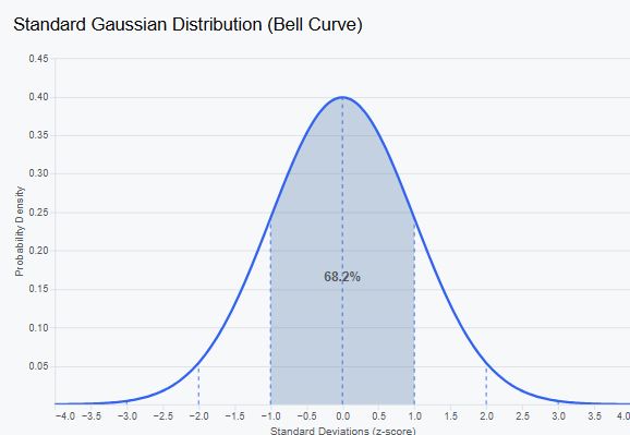
The Gaussian distribution (the normal distribution) is a continuous probability distribution that is symmetrical and shaped like a bell. It describes how data behaves in many real-world scenarios, from human heights to exam scores. 
The Gaussian distribution is uniquely important because The Central Limit Theorem (CLT) states that if you take large, random samples from any population (regardless of its original distribution shape), the distribution of the sample means will automatically approximate a Gaussian distribution as the sample size grows. This allows statisticians to make confident probability statements about populations even when the data looks chaotic.
Key Characteristics of the Bell Curve: The distribution is perfectly symmetrical around its center. The mean, median, and mode are all equal and located at the highest peak. 
A Gaussian distribution is entirely defined by two parameters:
The Mean (mu): The centre or average of the distribution.
The Standard Deviation (sigma): The measure of how spread out the data is. A smaller value makes the curve tall and narrow; a larger value makes it flat and wide. 
The 68-95-99.7 Rule. In a perfect Gaussian distribution, data falls within standard deviations of the mean in a highly predictable way: 
68.2% of the data falls within 1 standard deviation
95.4% of the data falls within 2 standard deviations
99.7% of the data falls within 3 standard deviations

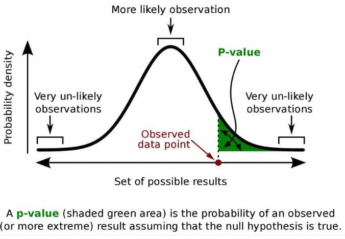
The primary measure of statistical significance is the p-value (probability value), which evaluates whether the results of an experiment or data sample are likely due to a specific cause rather than random chance.

Key Metrics of Significance Testing

• P-value: A value between 0 and 1 representing the probability of observing your data assuming that the null hypothesis is true (the assumption that there is no real effect or difference). [1, 2]
• Alpha Level (α): The prespecified threshold for significance, typically set before data collection. The standard threshold in most scientific research is 0.05 (5%).
• The Significance Rule: If the p-value is less than alpha (p < 0.05), the result is declared statistically significant. If it is greater, the results are considered explainable by chance alone.

What Statistical Significance Doesn't Measure
It is a common misconception that a highly statistically significant result means the finding is large or important. In reality:
It does not measure magnitude: A very small, trivial effect can be highly statistically significant if the sample size is large enough.
It requires Effect Size: To measure the actual strength or practical impact of a result, researchers use effect size metrics (such as Cohen's d or correlation coefficients) alongside the p-value.